2. Hybrid HMM/ANN speech recognition

2.1 Introduction

The continuous density hidden Markov model (CDHMM) is the dominant technology for automatic speech recognition today. However, a few significant limitations of the standard CDHMM suggest that other methods, or combinations of CDHMM with other methods, may improve the performance of the recognition. One class of such methods is based on artificial neural networks (ANNs). 
Speech recognition was one of the first problems that ANN models were applied to during the rapid spread of the methods in the 1980's. The complex mapping between the acoustic domain, and the set of  phonemes, has properties that are regarded to be modeled well with ANN methods. One reason for this is the good discriminative power of ANN models. 
ANN models have been used for word recognition directly (e.g., Ström, 1992; English and Boggess, 1992; Li, Naylor, and Rossen, 1992), but with limited success. It has been proven difficult to model the temporal aspects in an efficient manner within the ANN formalism. Combinations of an ANN with HMM that models most of the temporal constraints have been more successful. Several different methods have been proposed for combining the two. A few of the more well-known are: "Hybrid HMM/ANN Architecture" (Bourlard and Wellekens, 1988), "Linked Predictive Neural Networks" (Tebelskis and Waibel, 1990),  "Hidden Control Neural Architecture" (Levin, 1990), and "Stochastic Observation HMM" (Mitchel, Harper and Jamieson, 1996). 
The most successful architecture for combining CDHMM and ANN technology is currently the hybrid HMM/ANN model, where the ANN is utilized to estimate the observation probabilities of a CDHMM. This combination makes use of the discriminative power of the ANN approach, and relies on the HMM to model temporal aspects and the invocation of a probabilistic grammar. 
In this chapter, the hybrid system used in several of the included papers is reviewed. First the CDHMM that models the dynamic constrains imposed by the lexicon and grammar is discussed. Then I describe the ANN that models the mapping between acoustic observations and phonemes, and in section 2.5, sparse connection and pruning in the ANN are covered. 


2.2 The standard CDHMM

Although used for speech recognition, the HMM is most easily described as a speech production model. An HMM based speech recognizer has a set of different HMMs representing different units of speech, e.g., phonemes or words. The recognition process is a search to find the sequence of models that are the most likely to have produced the utterance. 
In the standard CDHMM formalism, the speech signal is assumed to be produced by a probabilistic finite state automaton (FSA). A graphic representation of an HMM, modeling a phoneme is shown in Figure 2. In the following I assume that all HMMs model phonemes or special segments such as pauses etc. The model produces the signal by emitting, at each state of the FSA, an output observation and then moving to a new state. The emission of observations occurs at equidistant time-points, typically every 10 ms, and the output observation is a random variable with a different probability density function for each state. Also the motion between the states is governed by statistical laws. The allowed transitions have transition probabilities associated with them such that some paths through the FSA are more likely than others. This is the only inherent duration modeling in the standard CDHMM. 
The output probability densities are typically modeled by mixtures of multivariate Gaussian probability distributions with diagonal covariance matrices. This functional form is selected mostly for its mathematical properties, and in the case of the choice of diagonal covariance matrices, to reduce computations. 
The observations are representations of the speech signals in the short time frame of circa 10 ms covered by each emission. A set of features, the feature vector, is computed for each frame. A popular basic feature vector is the so called cepstrum coefficients vector. The cepstrum coefficients are the cosine coefficients of the spectrum of the signal in the frame. Typically, the cepstrum features, the total energy in the frame, and the first and second time-derivatives of these features, are the components of the observation vectors modeled by the multivariate mixture of Gaussian probability distributions. The size of these observation vectors are typically around 40. The feature vector extraction is discussed in detail in Paper 3. 
The framework of the CDHMM makes it straight-forward to optimize the model parameters using well-known parameter estimation paradigms from statistic theory. In particular, the maximum likelihood (ML) method is used. In short, it means that the parameters of the model - the means, variances and mixture weights of the distributions, and the transition probabilities - should be chosen in such a way that the probability that the correct sequence of HMMs produced the utterances of a training database is maximized. Or put in another way, the probability that the training utterances were produced by the models is maximized. There exists a computationally efficient algorithm, the Baum-Welch algorithm, that performs this maximization in an iterative expectation-maximization (EM) procedure. Each iteration of the algorithm is guaranteed to increase the probability of the training utterances, and thus convergence is established. 
The ML training with Baum-Welch's algorithm is popular mostly because of its computational attractiveness, but it is actually optimizing the model's ability to produce speech, instead of recognizing it. Parameters computed by MAP (maximum a posteriori) estimation give the recognizer, at least in theory, better discrimination ability, but are harder to compute. In this paradigm, the probability of the correct string of symbols (phonemes or words) is maximized, given the observations. This is a more intuitive optimization criterion for a model to be used for recognition (see Figure 3)). 
A third alternative is to search for the parameters that minimize the actual error rate of the recognizer on the training data (minimum classification error, MCE). This is clearly the optimal training criterion, but this optimization is a much harder task than finding the ML parameters by Baum-Welch's algorithm or even MAP estimation. 
Speech recognition in the CDHMM framework, is typically a procedure of finding the sequence of HMMs that are the most likely to have produced the utterance to recognize. Because the number of models can be rather large, and even more importantly, the boundaries between the models are unknown, this search is a very large problem that is in general not possible to solve without approximations. In practice, some variation of the Viterbi approximation is virtually always employed for continuous speech recognition (see section 3.2). In this approximation it is assumed that the probability of one path through the HMMs has much higher probability than all other paths. It is very clear that this underlying assumption is often not justified, but once again it is the attractive computational properties of the so called Viterbi algorithm that has made it the standard decoding method for CDHMM. 
 
Figure 2 
Figure 2. Graphical representation of an HMM. The HMM has one "hidden" stochastic process and one observable stochastic process. At each point in time, the model "is" in one of its states. The hidden process is the sequence of states visited. This process is governed by the transition probabilities, pij in the figure, for moving from one state to another. The observable process is the outputted acoustic feature vector at each state. These vectors are mixtures of multivariate Gaussian stochastic variables (with density function j in the figure). This particular structure with three states and transitions from left to right, self-loops but no skips is typically used for phoneme models.    
 
Figure 3 
Figure 3. The difference between the maximum likelihood (ML) optimization criterion and the maximum a posteriori (MAP) criterion can be illustrated by this figure. In the ML framework, the probability of the produced acoustic realizations, given the symbols to recognize is optimized. In the MAP framework, the probability of the symbols is instead optimized given the acoustic realizations. 

2.3 Problems with the standard model

The weaknesses of the standard CDHMM model, touched upon in the previous section, have been pointed out by several authors (e.g., Bourlard and Morgan 1993; Robinson, 1994), and can be summarized in the following points: 
  1. Poor discrimination due to the fact that model parameters are estimated by maximum likelihood (ML) estimation instead of an estimation method that attempts to explicitly minimize the classification error. Examples of such estimation schemes are: minimum classification error (MCE), and maximum a posteriori (MAP) estimation. 
  2. The a priori choice of model topology, and in particular the choice of functional form of the statistical distributions, e.g., assuming that the emission probabilities for the acoustic observations are mixtures of multivariate Gaussian densities with diagonal covariance matrices. This choice is based on the mathematical properties of the family of distribution functions and is not necessarily optimal. 
  3. The so called Markov assumption that state sequences are first-order Markov chains, i.e., the probability density distributions depend only on the current state. 
  4. The correlation between successive acoustic observations is not acknowledged. Note that this is different from the previous point where the influence of the state sequence was considered. 
  5. There is a mismatch between the Baum-Welch training and evaluation of the HMMs because the Viterbi approximation is active only in the evaluation phase. 
Thus, it seems that we have a rather strong case against the HMM technology. However, during the history of the model, designers of state-of-the-art CDHMM recognition systems have addressed all the above points and found ways to reduce the negative effects of them. The effects of point (3) have been reduced by introducing context dependent models, e.g., tri-phones. Point (4) has been addressed by adding delta and delta-delta coefficients to the observation vector. Parameter-tying schemes have made it possible to train very general probability density functions that can solve problems due to point (2), and recently, the ML training scheme has been complemented with MAP training in response to point (1). 
To summarize the analysis of the weaknesses of the CDHMM: on the foundation of an initial model that seems rather inappropriate for the task, an increasingly complex and more accurate model has emerged through incremental refinement. It is noteworthy that the original motivation for the choice of model that leads to the discussed weaknesses was to keep computation down, but the subsequent improvements that partially solved the initial problems have increased the computational demands dramatically. This is true in particular for the many models needed for triphone modeling and the computationally demanding probability distribution functions used. Thus, the improvements go hand in hand with the rapid development of computers. 
Given the above, it is not self-evident that the CDHMM would be the choice of model if automatic speech recognition were to be reinvented today. But because of the complexity of the problem and the large research and development investments in the current technology, it is very difficult to make a competitive system based on a completely new framework. When Bourlard (1995) discusses the present situation in the ASR field, he characterizes the prevailing CDHMM architecture as a local optimum in the space of recognition systems. He argues that it is necessary to change the architecture in a manner that increases recognition error rates in the short run, but has potential of long term improvement, thus escaping from the local optimum. 
In the hybrid HMM/ANN architecture, the standard framework is kept intact, but the observation probabilities are computed by an ANN. This addresses point (1) and (2) above, by the selection of model and training paradigm chosen - ANNs put very weak a priori constraints on the distributions and are trained in the MAP paradigm. Point (5) is also neutralized because the Baum-Welch algorithm is not used, but many of the imperfections of the standard model remain, e.g., the Viterbi approximation and points (3) and (4). 


2.4 The artificial neural network

In the late 1980's it was pointed out by several authors that the output activities of ANNs trained with the back-propagation algorithm approximate the a posteriori class probabilities (Baum and Wilczek 1988; Bourlard and Wellekens, 1988; Gish, 1990; Richard and Lippman, 1991). In the case of an ANN trained to recognize phonemes, this means that the ANN estimates the probability of each phoneme given the acoustic observation vector. This observation is of fundamental importance for the theoretical justification of the hybrid HMM/ANN model. By application of Bayes' rule, it is easy to convert the a posteriori probabilities to observation likelihoods, i.e, 
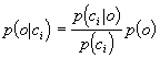
Equation 1
(1)
where ci  is the event that phoneme i is the correct phoneme, o is the acoustic observation, and p(ci) is the a priori likelihood of phoneme i. The unconditioned observation probability, p(o), is a constant for all phonemes and can consequently be dropped without changing the relative relation between phonemes, and the a priori phoneme probabilities are easily computed from relative frequencies in training speech data. Thus, equation (1) can be used to define output probability density functions of a CDHMM. 
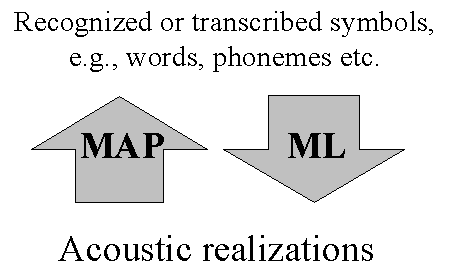
Back-propagation ANNs have intrinsically many of the features that have been added to the standard CDHMM in the development process discussed in the previous section. The normal back-propagation estimates MAP phoneme probabilities, not ML estimates that is the normal estimation method for CDHMM. As mentioned, MAP has better discrimination ability than ML, and is a more intuitive method to train a model for recognition. 
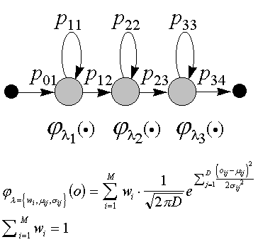
Also the parameter sharing/tying is available in the ANN at no extra cost. This was introduced in the CDHMM with added complexity as a consequence, to be able to use complex probability density functions without introducing too many free parameters. In Figure 4 it is seen that all output-units in the ANN share the intermediate results computed in the hidden units. However, this total sharing scheme can sometimes hurt performance and it is therefore beneficial to limit the sharing of hidden units. This is discussed more in section 2.5. 
The important short time dynamic features - formant transitions etc. - have been captured in ANNs by time-delayed connections between units (Waibel et al., 1987). This is a more general mechanism than the simple dynamic features (1st and 2nd time-derivatives) used in the standard CDHMM. One use of time-delayed connections is to let hidden units merge information from a window of acoustic observations, e.g., a number of frames centered at the frame to evaluate. The same mechanism can be used to feed the activity of the hidden units at past times, e.g., the previous time point, back to the hidden units. This yields recurrent networks that utilize contextual information by their internal memory in the hidden units (e.g., Robinson and Fallside, 1991). A general ANN architecture that encompasses both time delay windows and recurrency, is presented in Paper 6. 
Problems that are related to the HMM-part of the hybrid, are of course not solved by the introduction of the ANN. The Markov assumption, the Viterbi approximation etc. still remain. In many cases, the ad hoc solutions developed to reduce the effects of these problems for CDHMM can easily be translated to the hybrid environment, but in the case of context dependent models, e.g., tri-phones, there is an extra complication. It is not as straight-forward to apply Bayes' rule to the output activities when they are conditioned by the surrounding phoneme identities. It turns out that, to compute the observation likelihood in this case, the probability of the context given the observation is needed, i.e., 
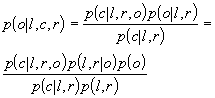
Equation 2
 (2)
where c is the phoneme, and l and r are the right and left context phonemes. This problem has been solved by (Bourlard and Morgan, 1993; Kershaw, Hochberg and Robinson, 1996) by introducing a separate set of output units for the context probabilities, p(l,r|o), but their results indicate that the gain with tri-phones is smaller for the hybrid model than for the standard CDHMM. 
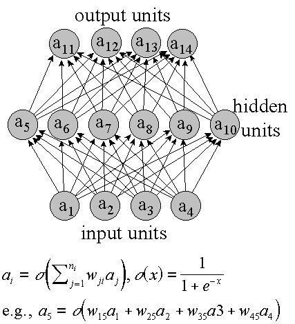
 
Figure 4 
Figure 4. Graphical representation of a feed-forward ANN. Associated with each node at each time is an activity. This is a real bounded number, e.g., [0; 1] or [-1; 1]. The activities of the input units is the input pattern to classify. The activities of all other units are computed by taking a weighted sum of the activities of the units in lower layers, and then applying a compressing function s to get a bounded value. The activities of the output units are the networks response to the input pattern. To train an ANN for a particular task, a training database is prepared with input patterns and corresponding target vectors for the output units. The weights, wij, of the ANN are adjusted to make the output units' activities as close as possible to the target values. This is done iteratively in the so called back-propagation training. 
 

 2.5 Sparse connection and pruning in the ANN

The number of hidden units determines to a large extent a network's ability to estimate the a posteriori probabilities accurately. One could argue that it is the number of free trainable parameters in the network that is the important factor. In this view, it is not the number of units, but the number of connections that is important. However, from experience we know that not only the number of parameters is important, but also how they are put to use. In large, fully-connected networks, the number of connections is several orders of magnitude higher than the number of units. This means that each unit has several hundred, sometimes thousands of in-flowing connections. It is unlikely that all these connections can provide useful information to the one-dimensional output of the unit. Also, by studying the distribution of the weights in trained ANNs it can be noted that there is a high concentration of weights close to zero. Therefore it can be advantageous to work with sparsely connected networks where units are connected only to a fraction of all units in higher layers. 
In Paper 6 I show that the ANN performance can be greatly increased by shifting the balance between the number of units and connections by introducing sparse connectivity. Two different approaches for achieving sparse connectivity are explored: connection pruning and sparse connection. 
Connection pruning is a method that is applied after the network is trained. The network is analyzed and each connection is given a measure of salience. A fraction of the connections with the smallest salience is then removed and the resulting, smaller ANN is retrained. The most well-known pruning criterion is due to Le Cun, Denker, and Solla (1990), and was given the imaginative name "Optimal Brain Damage". In this method the salience depends on the second derivative of the objective function of the back-propagation. In Paper 6, a more simplistic measure is used, the salience is simply the magnitude of the connection weight. 
In Paper 6, a reduction to about half the number of connections was found to be possible without significant performance degradation. The computational complexity for running the ANN is proportional to the number of connections. Thus, this may be of great importance when computation is critical. Since pruning reduces the number of free parameters, it can also improve the network's generalization ability (e.g. Le Cun, Denker and Solla, 1990; Sietsma and Dow, 1991), but since we used a truncated training that handles problems with over-adaptation to the training data, this potential benefit is less important in our case. 
Pruning the connections of an already trained network has no impact on the computational effort for training. To be able to apply the pruning criterion to the connections, the weights of the fully connected network must first be trained. Therefore, a second method - to start the training with already sparsely connected networks - was also explored in Paper 6. Before training, there is no available information about which connections are salient, so a random set of connections must be selected. Of course, this is in general not an optimal set, but the results show that sparsely connected ANNs perform much better than their fully connected counterparts with equal number of connections 
The continuous density hidden Markov model (CDHMM) is the dominant technology for automatic speech recognition today. However, a few significant limitations of the standard CDHMM suggest that other methods, or combinations of CDHMM with other methods, may improve the performance of the recognition. One class of such methods are based on artificial neural networks (ANNs).
Speech recognition was one of the first problems that ANN models were applied to during the rapid spread of the methods in the 1980's. The complex mapping between acoustic sounds and linguistic units such as phonemes has properties that are regarded to be modeled well with ANN methods. One reason is the good discriminative power of ANN models. 
ANN models have been used for word recognition directly (e.g., Ström, 1992; English and Boggess, 1992; Li, Naylor, and Rossen, 1992), but with limited success. It has been proven difficult to model the temporal aspects in an efficient manner within the ANN formalism. Combinations of an ANN with HMM that models most of the temporal constraints have been more successful. Several different methods have been proposed for combining the two. A few of the more well-known are: "Hybrid HMM/ANN Architecture" (Bourlard and Wellekens, 1988), "Linked Predictive Neural Networks" (Tebelskis and Waibel, 1990),  "Hidden Control Neural Architecture" (Levin, 1990), and "Stochastic Observation HMM" (Mitchel, Harper and Jamieson, 1996). 
The most successful architecture for combining CDHMM and ANN technology is currently the hybrid HMM/ANN model, where the ANN is utilized to estimate the observation probabilities of a CDHMM. This combination makes use of the discriminative power of the ANN approach, and relies on the HMM to model temporal aspects and the invocation of a probabilistic grammar. 
In this chapter, the hybrid used in several of the included papers is reviewed. First the CDHMM is discussed that models the dynamic constrains imposed by the lexicon and grammar. Then I describe the ANN that models the acoustic mapping between acoustic observations and phonemes, and in section 2.5, sparse connection and pruning in the ANN is covered.